Regions of Genomic Plasticity - panRGP
What is PPanGGOLiN ?
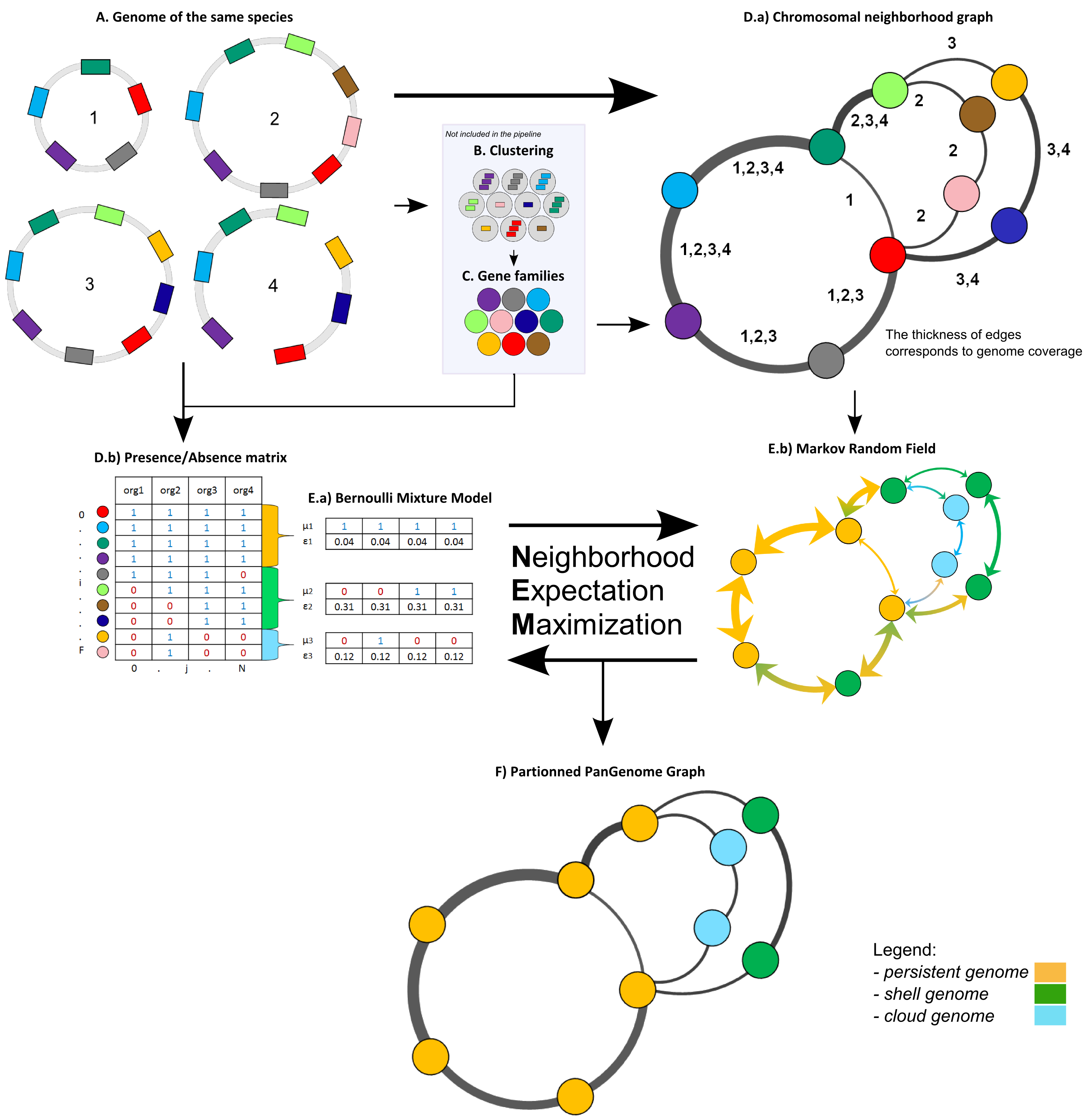
The panRGP tool uses the inputs of PPanGGOLiN software. PPanGGOLiN computes pangenomes for each MicroScope Genome Cluster (MICGC correspond to clusters of genomes from the same species) (A). It relies on a graph approach to modelize pangenomes in which nodes and edges represent families of homologous genes and genomic neighborhood information, respectively (B and C). Homologous families are from MICFAM computed with stringent parameters (80% of aa identity and 80% of alignment coverage). PPanGGOLiN approach takes into account both graph topology (D.a) and occurrences of genes (D.b) to classify gene families into three partitions (i.e. persistent genome, shell genome and cloud genome) yielding to what we called Partitioned Pangenome Graphs (F). More precisely, the method depends upon an Expectation/Maximization algorithm based on Bernoulli Mixture Model (E.a) coupled with a Markov Random field (E.b).
Pangenome Graph Partitions:
Persistent genome: equivalent to a relaxed core genome (genes conserved in almost all genomes).
Shell genome: genes having intermediate frequencies corresponding to moderately conserved genes (potentially associated to environmental adaptation capabilities).
Cloud genome: genes found at very low frequencies (potentially newly transferred genes).
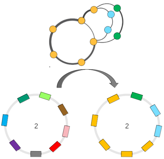
As illustrated below, the PPanGGOLiN classification can be projected on each genome of the analyzed MICGC:
More information about PPanGGOLiN is available here.
Warning
The panRGP tool is executed only on MICGC containing at least 15 strains. Please also note that we exclude genomes for which CheckM detected more than 5% contamination or less than 90% completeness as they are not assigned to MICGC cluster (see Genome Overview).
What is a Region of Genomic Plasticity (RGP) ?
A RGP is a region of a genome structurally not present in related others. RGPs can be sites of insertions of integrated Mobile Genetic Elements (MGE), or the result of deletions of particular segments of DNA in one or more strains. Therefore, the RGP designation does not make any assumption about the evolutionary origin or genetic basis of these variable chromosomal segments.
These regions are known to encode virulence, antimicrobial resistance factors and contains genes conferring specific adaptation functions (pathogenicity, symbiosis properties, detoxification …).
Reference:
What is a panRGP ?
The goal of panRGP is to efficiently detect RGPs within a partitioned pangenome graph. Based on the projection of the partitioned PPanGGOLiN graph on a given genome, the method defines as a RGP a set of consecutive genes that are members of the shell or cloud genomes.
The panRGP method browses the genes along the genome to determine the RGP boundaries using a score-based algorithm as shown in the figure below (persistent: yellow, shell: green, cloud: blue).
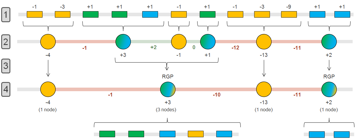
In steps 1 & 2, groups of consecutive persistent or shell/cloud genes are made and a score is computed. For groups of shell/cloud genes, the score corresponds to the number of genes. For persistent groups, the score is calculated as follow (where n is the number of consecutive persistent genes):

In steps 3 & 4, a persistent group is merged with its surrounding shell/cloud groups if its score (absolute value) is less than or equal to the minimum score of the neighboring shell/cloud groups. In this case, the persistent genes will be considered as part of the RGP. In this example, a RGP of 5 genes (3 shells, 1 persistent and 1 cloud) and one of 2 genes (2 clouds) are obtained.
Note
RGPs must be composed of at least 2 genes and have a minimum length of 5 kb to be detected.
How to access to panRGP data ?
panRGP predictions are available through the Comparative Genomics section, in the main navigation menu.
How to read the interface ?
In the genome cluster information table, you can find out which MICGC your organism belongs to and switch to another within the same genome cluster. The total number of organisms in the MICGC that were used to compute the RPGs is also indicated.
Note
You may not have access to all the organisms used to compute the RGPs, as some may have restricted access based on annotator access rights.
You can visualize the genome partition in a circular representation using CGView (see What is CGView?).
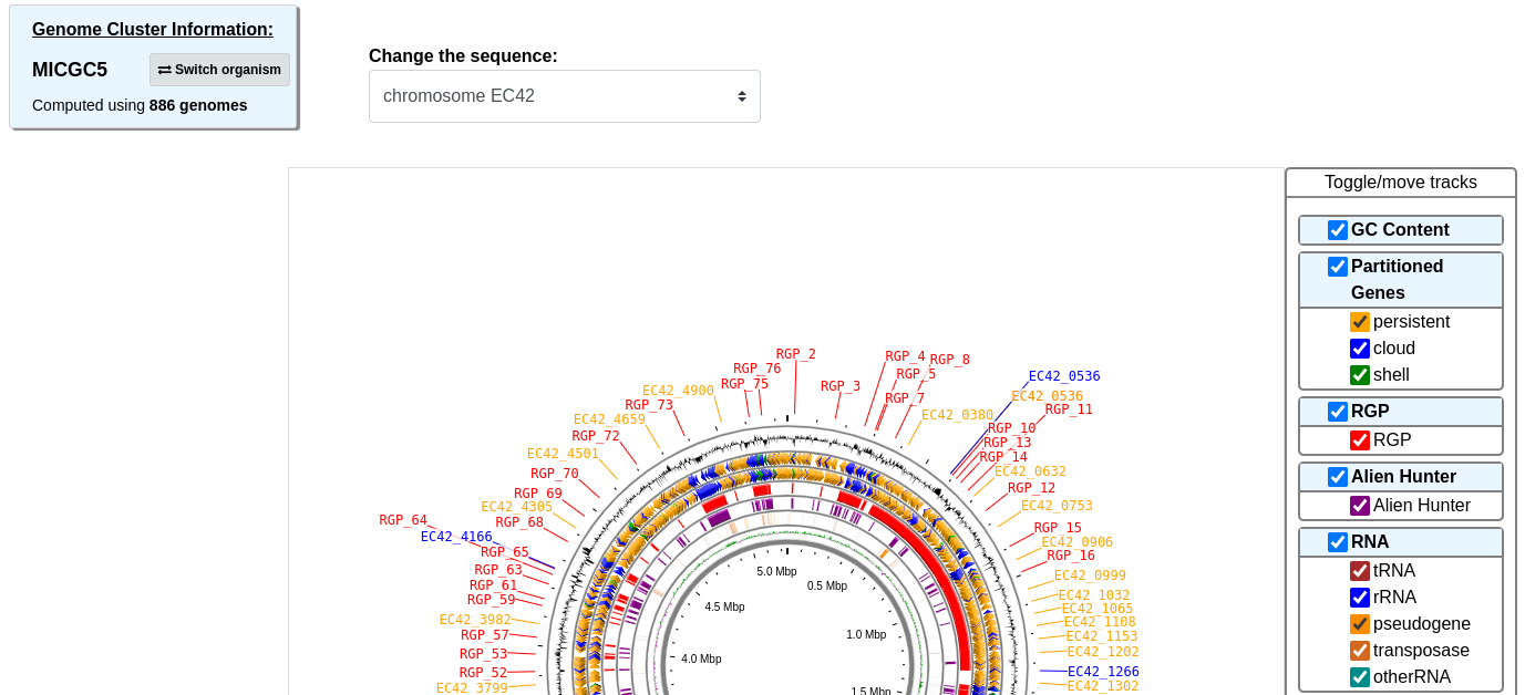
Tracks (from the outside):
GC Content
CDSs in the negative strand: yellow for persistent genome, green for shell genome and blue for cloud genome
CDSs in the positive strand (same color code as above)
Predicted RGPs (red)
Alien Hunter/IVOM results (purple)
tRNAs (green), rRNAs (blue), misc RNAs (grey), pseudogenes (sea green), transposases (chocolate) and others (orange)
GC Skew
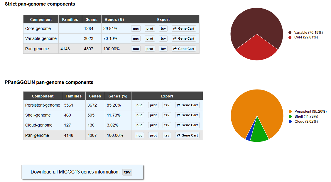
The “Strict pan-genome components” table represents a summary of the exact core-variable analysis.
The “PPanGGOLiN pan-genome components” table gives the number of genes and MICFAM families for each PPanGGOLiN partition.
You can extract all these genes in fasta format (nucleic and proteic), tsv with their annotation or in a gene card to do further analysis on them.
Finally, the “Regions of Genomic Plasticity” table gives you an overview of all the RGPs in the given organism that were predicted by the panRGP method.
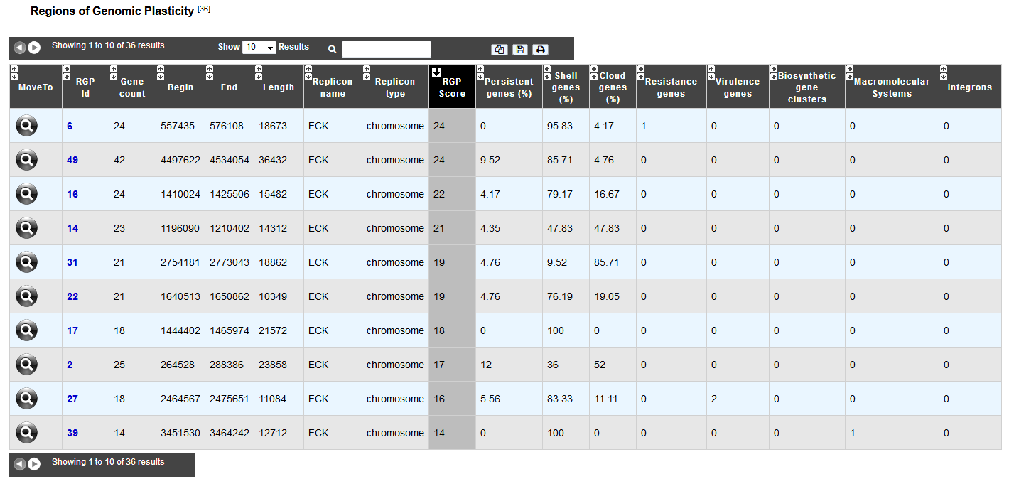
For each RGP, the number of genes predicted by other methods is indicated:
Resistance genes: Antibiotic resistance prediction using CARD method
Virulence genes: Virulence prediction
Biosythetic gene clusters: AntiSMASH Prediction
Macromolecular systems: MacSyFinder Prediction
Integrons: IntegronFinder Prediction
How to explore panRGP ?
The RGP visualization window can be accessed by clicking on any RGP number in the RGP id field. This window allows you to access to a detailed description of the RGP.